MaldiAMRKit - Exploration & Similarity

This notebook demonstrates how to use MaldiAMRKit’s exploratory visualisation and spectral similarity functions to inspect MALDI-TOF datasets before building classifiers.

It covers:

• PCA scatter plots coloured by metadata

• t-SNE embeddings

• UMAP embeddings (requires pip install maldiamrkit[batch])

• Spectral similarity: pairwise distance matrices, heatmaps, clustering, and dendrograms

• Brief introduction to batch effect correction with combatlearn

Dataset

This notebook uses the full multi-site version of the MALDI-Kleb-AI dataset (Rocchi et al., 2026; Zenodo DOI 10.5281/zenodo.17405072) - all three Italian centres (Rome, Milan, Catania), about 770 spectra. The other notebooks restrict themselves to the Rome sub-cohort, but exploration is precisely where you want the full multi-centre cohort: unsupervised methods will quickly tell you whether site / batch effects dominate the resistance signal. The helper in `notebooks/_demo.py <_demo.py>`__ caches the 370 MB tarball under ~/.cache/maldiamrkit/ on first use.

import pathlib
import sys

from maldiamrkit.visualization import plot_pca, plot_tsne

sys.path.insert(0, str(pathlib.Path.cwd()))  # _demo.py sits next to this notebook
from _demo import load_maldi_kleb_ai

/home/ettore/.venvs/maldiamrkit/lib/python3.10/site-packages/tqdm/auto.py:21: TqdmWarning: IProgress not found. Please update jupyter and ipywidgets. See https://ipywidgets.readthedocs.io/en/stable/user_install.html
  from .autonotebook import tqdm as notebook_tqdm

Load the Dataset

Exploration is the one notebook where the full multi-site cohort is more interesting than the Rome-only slice: with three acquisition centres (Rome, Milan, Catania) we can see whether unsupervised structure tracks the resistance phenotype or the acquisition site. Pass city=None to load all three centres.

ds = load_maldi_kleb_ai(antibiotic="Amikacin", city=None, verbose=True)
data = ds.maldi_set
labels = ds.meta["Amikacin"]
sites = ds.meta["City"]
print(f"Samples: {ds.X.shape[0]}, Features: {ds.X.shape[1]}")
print(f"Labels: {labels.value_counts().to_dict()}")
print(f"Sites:  {sites.value_counts().to_dict()}")

Processing spectra: 100%|██████████| 743/743 [00:00<00:00, 4637.49spectrum/s]

Samples: 741, Features: 6000
Labels: {'S': 372, 'R': 369}
Sites:  {'Rome': 470, 'Milan': 184, 'Catania': 87}

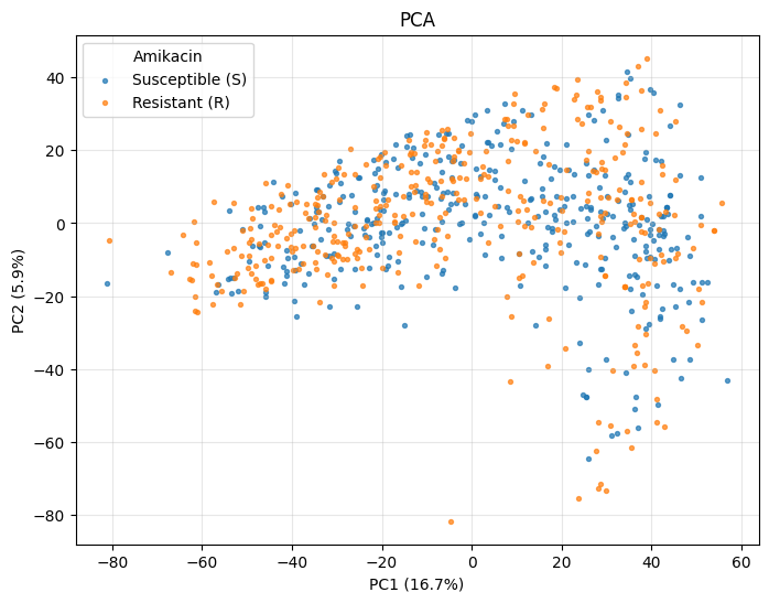
PCA

PCA is the simplest starting point. Axis labels automatically show the explained variance percentage.

_ = plot_pca(ds.X, color_by=labels)

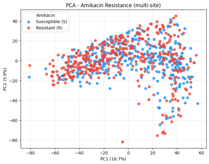
You can pass any matplotlib keyword arguments through **pca_kwargs, or provide a custom palette:

_ = plot_pca(
    ds.X,
    color_by=labels,
    palette={"S": "#2196F3", "R": "#F44336"},
    title="PCA - Amikacin Resistance (multi-site)",
    alpha=0.8,
    s=35,
)

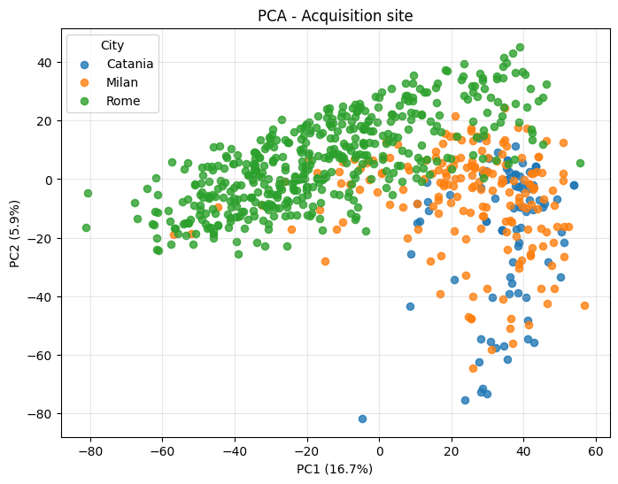
Now colour by the acquisition centre instead - if the three sites separate, you are seeing batch / instrument effects rather than biology, and the unsupervised plots are not telling you about resistance.

_ = plot_pca(
    ds.X,
    color_by=sites,
    title="PCA - Acquisition site",
    alpha=0.8,
    s=35,
)

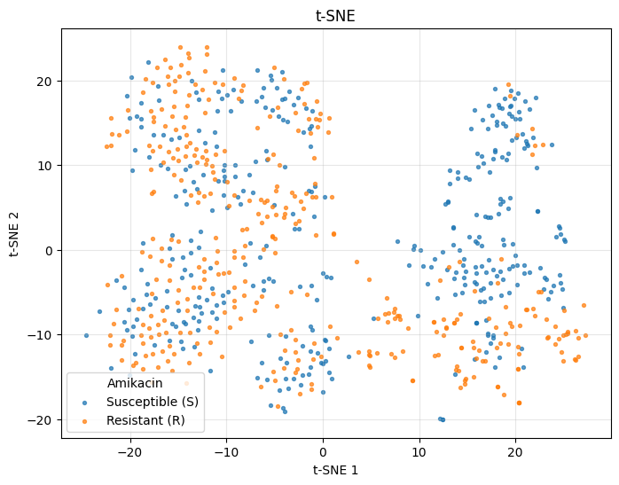
t-SNE

For a non-linear embedding, use plot_tsne. With ~470 samples, perplexity in the 20-40 range is a reasonable default.

_ = plot_tsne(ds.X, color_by=labels, perplexity=30, random_state=42)

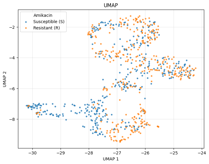
UMAP

UMAP requires the optional umap-learn package:

pip install maldiamrkit[batch]

try:
    from maldiamrkit.visualization import plot_umap

    _ = plot_umap(ds.X, color_by=labels, n_neighbors=15, random_state=42)
except ImportError as e:
    print(e)

/home/ettore/.venvs/maldiamrkit/lib/python3.10/site-packages/umap/umap_.py:1952: UserWarning: n_jobs value 1 overridden to 1 by setting random_state. Use no seed for parallelism.
  warn(

Spectral Similarity

MaldiAMRKit provides spectral distance metrics, pairwise distance matrix computation, clustering algorithms, and dedicated plots for similarity analysis.

Available metrics (see SpectralMetric):

• cosine - cosine distance (binned spectra)

• spectral_contrast_angle - spectral contrast angle (binned spectra)

• pearson - 1 - Pearson correlation (binned spectra)

• wasserstein - Wasserstein / earth mover’s distance (raw spectra)

• dtw - dynamic time warping distance (raw spectra)

For the pairwise heatmap and dendrogram we subsample to keep the figures readable; the same calls scale to the full 470-spectrum matrix.

from maldiamrkit.similarity import (
    cluster_metadata_concordance,
    cluster_spectra,
    hierarchical_clustering,
    pairwise_distances,
    plot_dendrogram,
    plot_distance_heatmap,
    silhouette_scores,
)

Pairwise Distance Matrix

Compute a symmetric distance matrix from the binned feature matrix. For binned spectra, cosine distance is a natural choice.

import numpy as np

rng = np.random.default_rng(0)
subset_idx = rng.choice(ds.X.shape[0], size=80, replace=False)
X_subset = ds.X.iloc[subset_idx]
labels_subset = labels.iloc[subset_idx]

D = pairwise_distances(X_subset, metric="cosine")
print(f"Distance matrix shape: {D.shape}")
print(f"Range: [{D[D > 0].min():.4f}, {D.max():.4f}]")

Distance matrix shape: (80, 80)
Range: [0.0449, 0.8068]

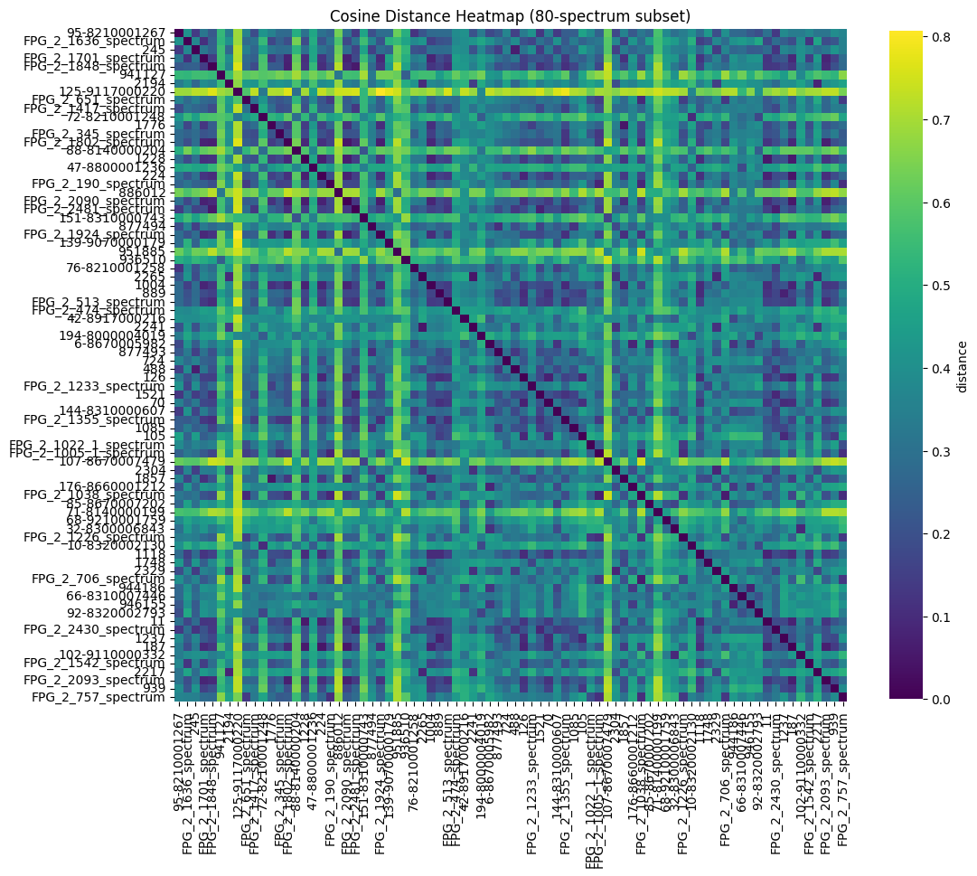
Distance Heatmap

Visualise the pairwise distance matrix. Darker values indicate more similar spectra.

_ = plot_distance_heatmap(
    D,
    labels=X_subset.index.tolist(),
    title="Cosine Distance Heatmap (80-spectrum subset)",
)

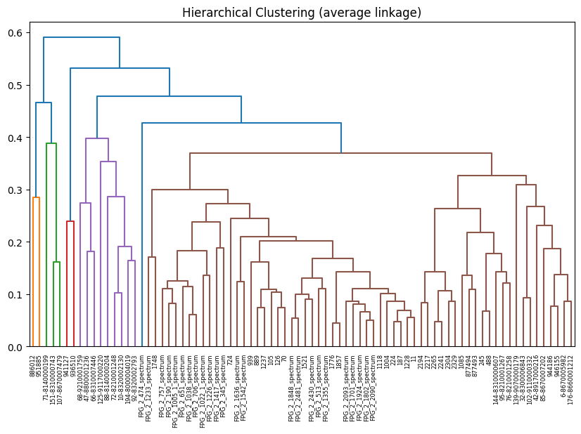
Hierarchical Clustering & Dendrogram

Build a linkage matrix and visualise the cluster hierarchy.

linkage = hierarchical_clustering(D, method="average")
_ = plot_dendrogram(
    linkage,
    labels=X_subset.index.tolist(),
    title="Hierarchical Clustering (average linkage)",
)

Cluster Assignment & Evaluation

Use cluster_spectra for a one-call clustering workflow. We ask for three clusters - matching the three acquisition centres - and then score the partition against both the resistance phenotype and the site label with silhouette scores and metadata concordance (ARI, NMI). This is a clean diagnostic: if clusters track the site but not the phenotype, batch effects are dominating the unsupervised signal - a classic motivator for ComBat-style correction.

We use method='kmedoids' here: with very uneven cluster sizes (Rome alone is ~470 spectra) average-linkage hierarchical clustering tends to peel off a couple of singletons instead of recovering the three centres. K-medoids respects the requested cluster count and produces balanced groups that closely match the site labels.

import pandas as pd

D_full = pairwise_distances(ds.X, metric="cosine")
cluster_labels = cluster_spectra(
    D_full,
    method="kmedoids",
    n_clusters=3,
    random_state=42,
)

sil = silhouette_scores(D_full, cluster_labels)
print(f"Silhouette score:               {sil:.3f}")

conc_pheno = cluster_metadata_concordance(cluster_labels, labels)
print("\nConcordance vs. Amikacin (R/S):")
print(f"  Adjusted Rand Index:          {conc_pheno['adjusted_rand_index']:.3f}")
print(f"  Normalized Mutual Info:       {conc_pheno['normalized_mutual_info']:.3f}")

conc_site = cluster_metadata_concordance(cluster_labels, sites)
print("\nConcordance vs. acquisition site (City):")
print(f"  Adjusted Rand Index:          {conc_site['adjusted_rand_index']:.3f}")
print(f"  Normalized Mutual Info:       {conc_site['normalized_mutual_info']:.3f}")

print("\nClusters x City:")
pd.crosstab(
    pd.Series(cluster_labels, index=sites.index, name="Cluster"),
    sites,
)

Silhouette score:               0.294

Concordance vs. Amikacin (R/S):
  Adjusted Rand Index:          0.029
  Normalized Mutual Info:       0.042

Concordance vs. acquisition site (City):
  Adjusted Rand Index:          0.688
  Normalized Mutual Info:       0.541

Clusters x City:

City	Catania	Milan	Rome
Cluster
0	7	7	439
1	80	110	21
2	0	67	10

Comparing Metrics

Try different distance metrics to see which one recovers the site structure most cleanly. We compare each metric against both the resistance phenotype and the acquisition site.

results = []
for metric in ["cosine", "spectral_contrast_angle", "pearson"]:
    D_m = pairwise_distances(ds.X, metric=metric)
    cl = cluster_spectra(D_m, method="kmedoids", n_clusters=3, random_state=42)
    sil_m = silhouette_scores(D_m, cl)
    conc_pheno = cluster_metadata_concordance(cl, labels)
    conc_site = cluster_metadata_concordance(cl, sites)
    results.append(
        {
            "metric": metric,
            "silhouette": sil_m,
            "ARI_pheno": conc_pheno["adjusted_rand_index"],
            "NMI_pheno": conc_pheno["normalized_mutual_info"],
            "ARI_site": conc_site["adjusted_rand_index"],
            "NMI_site": conc_site["normalized_mutual_info"],
        }
    )

pd.DataFrame(results).set_index("metric")

	silhouette	ARI_pheno	NMI_pheno	ARI_site	NMI_site
metric
cosine	0.294047	0.029394	0.041665	0.687924	0.541444
spectral_contrast_angle	0.152448	0.019211	0.016085	0.449982	0.410990
pearson	0.250229	0.016489	0.013949	0.391881	0.361815

Batch Effect Correction

When combining data from multiple sites or instruments, batch effects can dominate the signal. MaldiAMRKit on its own focuses on the single- site case (that is why this notebook restricts to Rome). For multi- centre harmonisation use combatlearn directly, or use the dedicated MaldiBatchKit sister package which builds on top of it:

from combatlearn import Combat

combat = Combat(method='fortin')
combat.fit(X, y=batch_labels)
X_corrected = combat.transform(X, y=batch_labels)

Install with pip install maldiamrkit[batch]. See the combatlearn documentation for full usage.

Rocchi, E., Nicitra, E., Calvo, M. et al. Combining mass spectrometry and machine learning models for predicting Klebsiella pneumoniae antimicrobial resistance: a multicenter experience from clinical isolates in Italy. BMC Microbiol (2026). doi:10.1186/s12866-025-04657-2