
MaldiAMRKit - Evaluation & Splitting#
This notebook covers AMR-specific evaluation metrics, stratified splitting utilities, and integration with scikit-learn’s cross-validation tools.
Dataset#
These notebooks use the MALDI-Kleb-AI dataset (Rocchi et al., 2026; Zenodo DOI 10.5281/zenodo.17405072), a curated archive of MALDI-TOF spectra of Klebsiella clinical isolates from three Italian centres (Rome, Milan, Catania) with Amikacin / Meropenem resistance annotations. For simplicity we restrict the demo to the Rome sub-cohort (single site, no batch correction needed). The helper in `notebooks/_demo.py <_demo.py>`__ caches the 370
MB tarball under ~/.cache/maldiamrkit/ (or $MALDIAMRKIT_CACHE_DIR) on first use.
Import Libraries#
[ ]:
import numpy as np
import pandas as pd
from sklearn.linear_model import LogisticRegression
from sklearn.model_selection import StratifiedKFold, cross_val_score
from sklearn.pipeline import Pipeline
from sklearn.preprocessing import StandardScaler

from maldiamrkit.evaluation import (
    CaseGroupedKFold,
    SpeciesDrugStratifiedKFold,
    amr_classification_report,
    case_based_split,
    categorical_agreement,
    major_error_rate,
    me_scorer,
    sensitivity_score,
    specificity_score,
    stratified_species_drug_split,
    very_major_error_rate,
    vme_me_curve,
    vme_scorer,
)
from maldiamrkit.susceptibility import LabelEncoder
AMR Evaluation Metrics#
In clinical antimicrobial resistance testing, standard ML metrics (accuracy, F1) do not capture the clinical severity of errors. MaldiAMRKit provides domain-specific metrics following EUCAST conventions:
VME (Very Major Error): resistant isolate called susceptible - the most dangerous error (could lead to treatment failure)
ME (Major Error): susceptible isolate called resistant - wasteful but not immediately dangerous
Sensitivity: TP / (TP + FN) = 1 - VME
Specificity: TN / (TN + FP) = 1 - ME
Categorical Agreement: overall accuracy (TP + TN) / N
We illustrate the metric definitions with a small hand-crafted vector so the arithmetic is easy to follow, then move on to a full run on the real dataset.
[2]:
# Toy 10-sample example for illustrating the metric definitions
y_true = np.array([1, 1, 1, 1, 0, 0, 0, 0, 0, 0])
y_pred = np.array([1, 1, 0, 1, 0, 0, 1, 0, 0, 0])

# Very Major Error: 1 out of 4 resistant samples was missed
vme = very_major_error_rate(y_true, y_pred)
print(f"VME (Very Major Error):   {vme:.2%}")

# Major Error: 1 out of 6 susceptible samples was falsely called resistant
me = major_error_rate(y_true, y_pred)
print(f"ME (Major Error):         {me:.2%}")

# Sensitivity and specificity
print(f"Sensitivity:              {sensitivity_score(y_true, y_pred):.2%}")
print(f"Specificity:              {specificity_score(y_true, y_pred):.2%}")

# Categorical agreement
print(f"Categorical Agreement:    {categorical_agreement(y_true, y_pred):.2%}")
VME (Very Major Error):   25.00%
ME (Major Error):         16.67%
Sensitivity:              75.00%
Specificity:              83.33%
Categorical Agreement:    80.00%
AMR Classification Report#
Get all metrics in a single dictionary with amr_classification_report.
[3]:
report = amr_classification_report(y_true, y_pred)
for key, value in report.items():
    if isinstance(value, float):
        print(f"  {key:>25s}: {value:.4f}")
    else:
        print(f"  {key:>25s}: {value}")
                        vme: 0.2500
                         me: 0.1667
                sensitivity: 0.7500
                specificity: 0.8333
      categorical_agreement: 0.8000
                n_resistant: 4
              n_susceptible: 6
                    n_total: 10
Load the Dataset#
Everything below runs on the real MALDI-Kleb-AI Rome cohort. The first call downloads 370 MB; later calls are instantaneous.
[4]:
import pathlib
import sys

sys.path.insert(0, str(pathlib.Path.cwd()))  # _demo.py sits next to this notebook
from _demo import load_maldi_kleb_ai

ds = load_maldi_kleb_ai(antibiotic="Amikacin", verbose=True)
ds.info
Processing spectra: 100%|██████████| 472/472 [00:00<00:00, 4855.36spectrum/s]
[4]:
{'source': 'Zenodo MALDI-Kleb-AI',
 'doi': '10.5281/zenodo.17405072',
 'record_id': '17405072',
 'md5_tar': 'c14b6c6b4210553962faa7f1dc27d275',
 'n_samples': 470,
 'n_bins': 6000,
 'bin_width': 3,
 'antibiotic': 'Amikacin',
 'city': 'Rome',
 'cache_dir': '/home/ettore/.cache/maldiamrkit/maldi-kleb-ai'}
[5]:
# Drop species with fewer than 2 samples - stratified splits need >=2
species_counts = ds.meta["Species"].value_counts()
keep = ds.meta["Species"].isin(species_counts[species_counts >= 2].index)

X = ds.X.loc[keep]
species = ds.meta.loc[keep, "Species"].values

enc = LabelEncoder(intermediate="susceptible")  # binary R vs rest
y = enc.fit_transform(ds.meta.loc[keep, "Amikacin"].values)

print(f"X shape: {X.shape}")
print(f"Class counts: {pd.Series(y).value_counts().to_dict()}")
print(f"Species: {pd.Series(species).value_counts().to_dict()}")
X shape: (469, 6000)
Class counts: {1: 272, 0: 197}
Species: {'Klebsiella pneumoniae': 469}
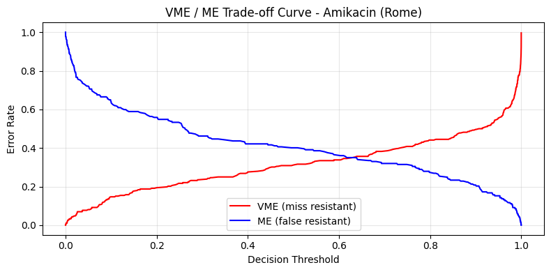
VME / ME Trade-off Curve on Real Predictions#
The vme_me_curve function computes VME and ME rates at varying decision thresholds. This is analogous to an ROC curve but uses clinically meaningful error types. We fit a quick logistic-regression baseline and read its out-of-fold probability scores.
[6]:
import matplotlib.pyplot as plt
from sklearn.model_selection import cross_val_predict

pipe = Pipeline(
    [
        ("scaler", StandardScaler()),
        ("clf", LogisticRegression(max_iter=2000, class_weight="balanced")),
    ]
)
cv = StratifiedKFold(n_splits=5, shuffle=True, random_state=42)
y_scores = cross_val_predict(pipe, X.values, y, cv=cv, method="predict_proba")[:, 1]

vme_rates, me_rates, thresholds = vme_me_curve(y, y_scores)

fig, ax = plt.subplots(figsize=(8, 4))
ax.plot(thresholds, vme_rates, "r-", label="VME (miss resistant)")
ax.plot(thresholds, me_rates, "b-", label="ME (false resistant)")
ax.set_xlabel("Decision Threshold")
ax.set_ylabel("Error Rate")
ax.set_title("VME / ME Trade-off Curve - Amikacin (Rome)")
ax.legend()
ax.set_ylim(-0.05, 1.05)
ax.grid(alpha=0.3)
plt.tight_layout()
plt.show()
Splitting Utilities#
Standard random splitting can cause data leakage or imbalanced species representation. MaldiAMRKit provides:
``stratified_species_drug_split``: stratified train/test split preserving species-drug label distributions
``case_based_split``: keeps all samples from the same patient in the same split to prevent leakage
Stratified Species-Drug Split#
[7]:
X_train, X_test, y_train, y_test = stratified_species_drug_split(
    X, y, species, test_size=0.2, random_state=42
)

print(f"Train: {len(X_train)} samples, Test: {len(X_test)} samples")
print(f"Train R-S: {y_train.sum():.0f}R - {len(y_train) - y_train.sum():.0f}S")
print(f"Test  R-S: {y_test.sum():.0f}R - {len(y_test) - y_test.sum():.0f}S")
Train: 375 samples, Test: 94 samples
Train R-S: 217R - 158S
Test  R-S: 55R - 39S
Case-Based Split#
In clinical data, multiple spectra may come from the same patient. case_based_split ensures no patient appears in both train and test sets.
The Zenodo metadata does not expose patient IDs, so we simulate them here by grouping every three consecutive spectra into one synthetic patient. In your own datasets, pass the real patient ID column.
[8]:
case_ids = np.array([f"patient_{i // 3}" for i in range(len(X))])

X_train_c, X_test_c, y_train_c, y_test_c = case_based_split(
    X, y, case_ids, test_size=0.3, random_state=42
)

train_pos = X.index.get_indexer(X_train_c.index)
test_pos = X.index.get_indexer(X_test_c.index)
train_cases = set(case_ids[train_pos])
test_cases = set(case_ids[test_pos])
print(f"Train: {len(X_train_c)} samples ({len(train_cases)} cases)")
print(f"Test:  {len(X_test_c)} samples ({len(test_cases)} cases)")
print(f"Case overlap: {len(train_cases & test_cases)} (should be 0)")
Train: 325 samples (109 cases)
Test:  144 samples (48 cases)
Case overlap: 0 (should be 0)
Cross-Validation Splitters#
MaldiAMRKit provides sklearn-compatible CV splitters for use with cross_val_score, GridSearchCV, etc.
``SpeciesDrugStratifiedKFold``: stratified by species-drug combinations
``CaseGroupedKFold``: grouped by patient/case ID
[9]:
cv_stratified = SpeciesDrugStratifiedKFold(n_splits=5, shuffle=True, random_state=42)

print("SpeciesDrugStratifiedKFold folds:")
for i, (train_idx, test_idx) in enumerate(
    cv_stratified.split(X.values, y, species=species)
):
    print(
        f"  Fold {i + 1}: train={len(train_idx)}, test={len(test_idx)}, "
        f"test R%={y[test_idx].mean():.1%}"
    )
SpeciesDrugStratifiedKFold folds:
  Fold 1: train=375, test=94, test R%=58.5%
  Fold 2: train=375, test=94, test R%=58.5%
  Fold 3: train=375, test=94, test R%=57.4%
  Fold 4: train=375, test=94, test R%=57.4%
  Fold 5: train=376, test=93, test R%=58.1%
[10]:
cv_grouped = CaseGroupedKFold(n_splits=5)

print("CaseGroupedKFold folds:")
for i, (train_idx, test_idx) in enumerate(
    cv_grouped.split(X.values, y, groups=case_ids)
):
    overlap = set(case_ids[train_idx]) & set(case_ids[test_idx])
    print(
        f"  Fold {i + 1}: train={len(train_idx)}, test={len(test_idx)}, "
        f"case overlap={len(overlap)}"
    )
CaseGroupedKFold folds:
  Fold 1: train=375, test=94, case overlap=0
  Fold 2: train=373, test=96, case overlap=0
  Fold 3: train=376, test=93, case overlap=0
  Fold 4: train=376, test=93, case overlap=0
  Fold 5: train=376, test=93, case overlap=0
sklearn Scorers#
Use vme_scorer and me_scorer directly with cross_val_score or GridSearchCV to optimise models for clinical error rates.
The scorers return negative values because sklearn maximises scores, and we want to minimise VME and ME.
[11]:
cv = StratifiedKFold(n_splits=5, shuffle=True, random_state=42)

auc_scores = cross_val_score(pipe, X, y, cv=cv, scoring="roc_auc")
print(f"ROC AUC:  {auc_scores.mean():.3f} +/- {auc_scores.std():.3f}")

vme_scores = cross_val_score(pipe, X, y, cv=cv, scoring=vme_scorer)
print(
    f"VME:      {vme_scores.mean():.3f} +/- {vme_scores.std():.3f}  (negative = better)"
)

me_scores = cross_val_score(pipe, X, y, cv=cv, scoring=me_scorer)
print(
    f"ME:       {me_scores.mean():.3f} +/- {me_scores.std():.3f}  (negative = better)"
)
ROC AUC:  0.714 +/- 0.029
VME:      -0.312 +/- 0.024  (negative = better)
ME:       -0.402 +/- 0.066  (negative = better)
Stratified CV + AMR Scorers#
Combine the domain-specific splitters with the AMR scorers for a complete clinical evaluation workflow.
[12]:
cv_clinical = SpeciesDrugStratifiedKFold(n_splits=5, shuffle=True, random_state=42)

vme_scores = cross_val_score(
    pipe,
    X.values,
    y,
    cv=cv_clinical.split(X.values, y, species=species),
    scoring=vme_scorer,
)
me_scores = cross_val_score(
    pipe,
    X.values,
    y,
    cv=cv_clinical.split(X.values, y, species=species),
    scoring=me_scorer,
)

print("Stratified CV with AMR scorers:")
print(f"  VME: {vme_scores.mean():.3f} +/- {vme_scores.std():.3f}")
print(f"  ME:  {me_scores.mean():.3f} +/- {me_scores.std():.3f}")
Stratified CV with AMR scorers:
  VME: -0.312 +/- 0.024
  ME:  -0.402 +/- 0.066