MaldiAMRKit - Drift Monitoring

This notebook demonstrates maldiamrkit.drift.DriftMonitor, which anchors a baseline on the earliest timestamps and tracks temporal drift through three complementary views:

• Reference similarity - distance of per-window median spectrum to the baseline reference (no labels needed)

• PCA centroid trajectory - how windows move in a baseline-fitted PCA space

• Peak-selection stability + effect-size drift - Jaccard overlap of top-k discriminative peaks per window vs. baseline, and Cohen’s d of specific peaks over time

Dataset

These notebooks use the MALDI-Kleb-AI dataset (Rocchi et al., 2026; Zenodo DOI 10.5281/zenodo.17405072), a curated archive of MALDI-TOF spectra of Klebsiella clinical isolates from three Italian centres (Rome, Milan, Catania) with Amikacin / Meropenem resistance annotations. For simplicity we restrict the demo to the Rome sub-cohort (single site, no batch correction needed). The helper in `notebooks/_demo.py <_demo.py>`__ caches the 370 MB tarball under ~/.cache/maldiamrkit/ (or $MALDIAMRKIT_CACHE_DIR) on first use.

Load the Dataset

We load the Rome cohort. The Zenodo metadata does not expose an acquisition timestamp, so we simulate dates by spreading the real spectra uniformly across a six-month window. The spectra themselves are real clinical isolates; only the time axis is synthetic, which lets us demonstrate the DriftMonitor API end-to-end without fabricating data.

import pathlib
import sys

import numpy as np
import pandas as pd

from maldiamrkit.susceptibility import LabelEncoder

sys.path.insert(0, str(pathlib.Path.cwd()))  # _demo.py sits next to this notebook
from _demo import load_maldi_kleb_ai

ds = load_maldi_kleb_ai(antibiotic="Amikacin", verbose=True)
encoder = LabelEncoder(intermediate="nan")
y = (
    pd.Series(
        encoder.fit_transform(ds.meta["Amikacin"]),
        index=ds.meta.index,
        name="Amikacin",
    )
    .dropna()
    .astype(int)
)
X = ds.X.loc[y.index]
print(f"Rows: {X.shape}, class counts: {y.value_counts().to_dict()}")

/home/ettore/.venvs/maldiamrkit/lib/python3.10/site-packages/tqdm/auto.py:21: TqdmWarning: IProgress not found. Please update jupyter and ipywidgets. See https://ipywidgets.readthedocs.io/en/stable/user_install.html
  from .autonotebook import tqdm as notebook_tqdm
Processing spectra: 100%|██████████| 472/472 [00:00<00:00, 4947.34spectrum/s]

Rows: (470, 6000), class counts: {1: 273, 0: 197}

Attach a Synthetic Acquisition Date

We spread the spectra evenly across 180 days, ordered by sample ID, and wrap them in a tiny shim exposing .X, .meta, and .get_y_single()

• the only attributes DriftMonitor needs.

from dataclasses import dataclass


@dataclass
class TimestampedSet:
    """Adapter that exposes the small surface DriftMonitor expects."""

    X: pd.DataFrame
    meta: pd.DataFrame

    def get_y_single(self, antibiotic: str | None = None) -> pd.Series:
        """Return the label column for ``antibiotic`` (default Amikacin)."""
        col = antibiotic or "Amikacin"
        return self.meta.loc[self.X.index, col]


ordered = X.sort_index()
start = pd.Timestamp("2025-01-01")
days = np.linspace(0, 180, num=len(ordered), dtype=int)
dates = [start + pd.Timedelta(days=int(d)) for d in days]

meta_full = pd.DataFrame(
    {
        "Amikacin": y.loc[ordered.index].astype(int),
        "acquisition_date": dates,
    },
    index=ordered.index,
)
dataset = TimestampedSet(X=ordered, meta=meta_full)
lo = meta_full["acquisition_date"].min().date()
hi = meta_full["acquisition_date"].max().date()
print(f"Date range: {lo} → {hi}")
print("Class counts:", meta_full["Amikacin"].value_counts().to_dict())

Date range: 2025-01-01 → 2025-06-30
Class counts: {1: 273, 0: 197}

Fit the DriftMonitor

By default, the baseline is the earliest 20% of sorted timestamps. Below we use a 30-day sliding window.

from maldiamrkit.drift import DriftMonitor

monitor = DriftMonitor(
    time_column="acquisition_date",
    window="30D",
    metric="cosine",
    min_samples=5,
).fit(dataset)
print(f"Baseline cutoff: {monitor.baseline_end_.date()}")

Baseline cutoff: 2025-02-05

1. Reference Similarity

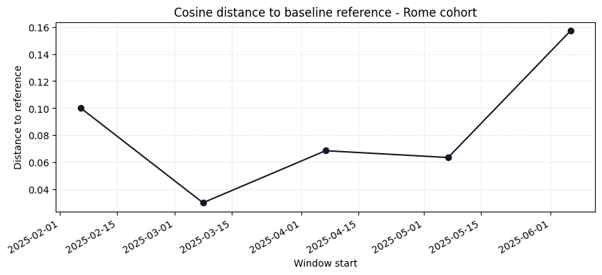
For each 30-day window we compute the median spectrum and measure its cosine distance to the baseline reference (element-wise median of baseline rows). A rising line signals that the population is drifting away from the baseline fingerprint.

from maldiamrkit.drift import plot_reference_drift

ref_df = monitor.monitor(dataset)
ref_df.head()

	window_start	window_end	n_spectra	distance_to_reference
0	2025-02-06	2025-03-08	78	0.100245
1	2025-03-08	2025-04-07	79	0.030005
2	2025-04-07	2025-05-07	78	0.068501
3	2025-05-07	2025-06-06	78	0.063464
4	2025-06-06	2025-07-06	63	0.157319

_ = plot_reference_drift(
    ref_df,
    title="Cosine distance to baseline reference - Rome cohort",
)

2. PCA Centroid Trajectory

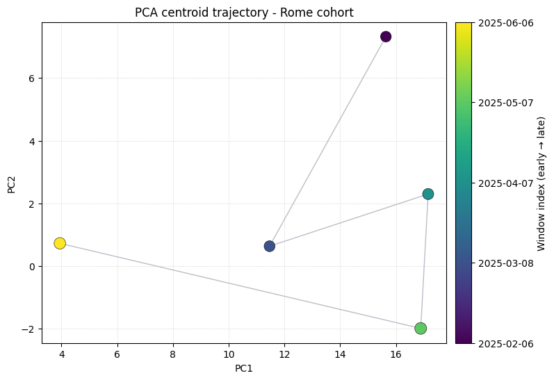
monitor_pca projects each window’s rows onto a PCA space fitted on the baseline, then reports the per-window centroid (PC1, PC2) and dispersion (mean distance from centroid).

plot_pca_drift draws arrows between consecutive centroids and colours each point by time (early → late).

from maldiamrkit.drift import plot_pca_drift

pca_df = monitor.monitor_pca(dataset)
pca_df.head()

	window_start	window_end	centroid_pc1	centroid_pc2	dispersion	n_spectra
0	2025-02-06	2025-03-08	15.638410	7.322260	28.561470	78
1	2025-03-08	2025-04-07	11.465971	0.634700	29.147355	79
2	2025-04-07	2025-05-07	17.153615	2.299735	30.926929	78
3	2025-05-07	2025-06-06	16.887356	-1.988096	35.732134	78
4	2025-06-06	2025-07-06	3.947033	0.726848	33.505330	63

_ = plot_pca_drift(pca_df, title="PCA centroid trajectory - Rome cohort")

3. Peak-Selection Stability

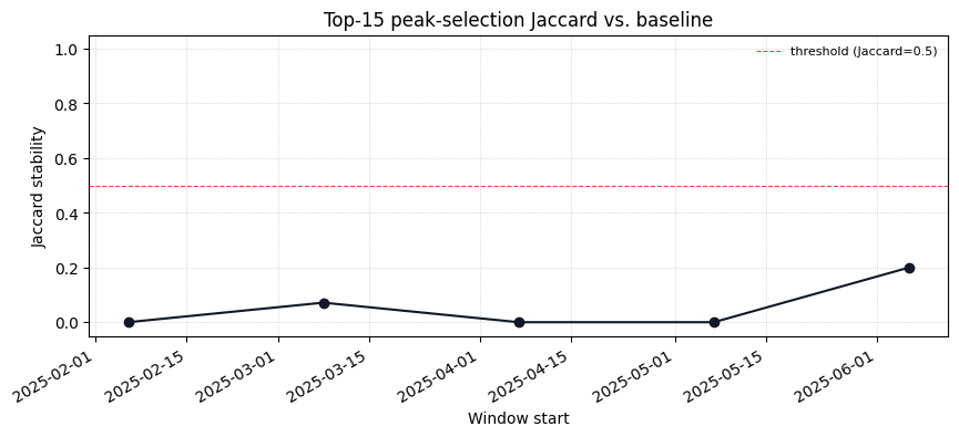
For each window, monitor_peak_stability fits a fresh DifferentialAnalysis and computes the Jaccard overlap of its top-k peaks with the baseline top-k. A falling curve means discriminative peaks are shifting over time - a red flag for biomarker studies.

from maldiamrkit.differential import DifferentialAnalysis
from maldiamrkit.drift import plot_peak_stability

baseline_analysis = DifferentialAnalysis(ordered, meta_full["Amikacin"]).run()
stability_df = monitor.monitor_peak_stability(
    dataset,
    baseline_analysis,
    antibiotic="Amikacin",
    n_top=15,
)
stability_df.head()

	window_start	stability_score	n_spectra
0	2025-02-06	0.000000	78
1	2025-03-08	0.071429	79
2	2025-04-07	0.000000	78
3	2025-05-07	0.000000	78
4	2025-06-06	0.200000	63

_ = plot_peak_stability(
    stability_df,
    title="Top-15 peak-selection Jaccard vs. baseline",
)

4. Per-Peak Effect-Size Drift

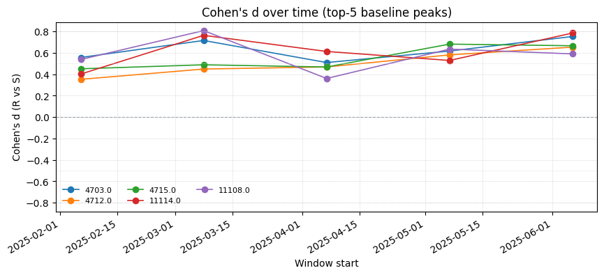
If you already have a short list of peaks of interest (e.g., from the baseline analysis), monitor_effect_sizes tracks their Cohen’s d between R and S in each window. A peak whose d drops toward zero (or flips sign) is losing discriminative power.

from maldiamrkit.drift import plot_effect_size_drift

top5 = baseline_analysis.top_peaks(n=5)["mz_bin"].astype(str).tolist()
effect_df = monitor.monitor_effect_sizes(
    dataset,
    peaks=top5,
    antibiotic="Amikacin",
)
effect_df.head()

	window_start	4703.0	4712.0	4715.0	11114.0	11108.0
0	2025-02-06	0.556368	0.352241	0.450814	0.401412	0.537368
1	2025-03-08	0.715240	0.448572	0.488254	0.763298	0.807354
2	2025-04-07	0.509200	0.468215	0.467595	0.612715	0.360646
3	2025-05-07	0.616484	0.580740	0.681273	0.528699	0.634580
4	2025-06-06	0.752635	0.653076	0.665924	0.785004	0.589966

_ = plot_effect_size_drift(
    effect_df,
    title="Cohen's d over time (top-5 baseline peaks)",
)

See Also

• API Reference - Drift

• Differential Analysis notebook for the DifferentialAnalysis class that monitor_peak_stability reuses internally.