MaldiAMRKit - Differential Analysis

This notebook demonstrates the maldiamrkit.differential module for identifying m/z bins that differ significantly between resistant (R) and susceptible (S) groups, and for comparing significant peaks across multiple drugs.

It covers:

• DifferentialAnalysis on a binned feature matrix (Mann-Whitney U or Welch’s t-test)

• Multiple-testing correction (FDR-BH, FDR-BY, Bonferroni), log2 fold change, Cohen’s d

• Ranking peaks with top_peaks() and filtering with significant_peaks()

• AMR-aware plots: plot_volcano, plot_manhattan

• Multi-drug comparison via compare_drugs + plot_drug_comparison (heatmap / UpSet)

Dataset

These notebooks use the MALDI-Kleb-AI dataset (Rocchi et al., 2026; Zenodo DOI 10.5281/zenodo.17405072), a curated archive of MALDI-TOF spectra of Klebsiella clinical isolates from three Italian centres (Rome, Milan, Catania) with Amikacin / Meropenem resistance annotations. For simplicity we restrict the demo to the Rome sub-cohort (single site, no batch correction needed). The helper in `notebooks/_demo.py <_demo.py>`__ caches the 370 MB tarball under ~/.cache/maldiamrkit/ (or $MALDIAMRKIT_CACHE_DIR) on first use.

Load the Dataset

We load the Rome cohort and use LabelEncoder(intermediate='drop') to build a binary label vector. The Zenodo dataset also ships a Meropenem annotation, which we will use later for the multi-drug comparison.

import pathlib
import sys

import pandas as pd

from maldiamrkit.susceptibility import LabelEncoder

sys.path.insert(0, str(pathlib.Path.cwd()))  # _demo.py sits next to this notebook
from _demo import load_maldi_kleb_ai

ds = load_maldi_kleb_ai(antibiotic="Amikacin", verbose=True)
encoder = LabelEncoder(intermediate="nan")  # map 'I' to NaN so lengths stay aligned
y = (
    pd.Series(
        encoder.fit_transform(ds.meta["Amikacin"]),
        index=ds.meta.index,
        name="Amikacin",
    )
    .dropna()
    .astype(int)
)
X = ds.X.loc[y.index]
print(f"X shape: {X.shape}")
print(f"Class counts: {y.value_counts().to_dict()}")

/home/ettore/.venvs/maldiamrkit/lib/python3.10/site-packages/tqdm/auto.py:21: TqdmWarning: IProgress not found. Please update jupyter and ipywidgets. See https://ipywidgets.readthedocs.io/en/stable/user_install.html
  from .autonotebook import tqdm as notebook_tqdm

Processing spectra:   0%|          | 0/472 [00:00<?, ?spectrum/s]
Processing spectra:  98%|█████████▊| 464/472 [00:00<00:00, 4632.35spectrum/s]
Processing spectra: 100%|██████████| 472/472 [00:00<00:00, 4600.71spectrum/s]

X shape: (470, 6000)
Class counts: {1: 273, 0: 197}

Run the Differential Analysis

Instantiate DifferentialAnalysis with X and y and call .run(). The default test is Mann-Whitney U (non-parametric, recommended for MALDI peak intensities) with Benjamini-Hochberg FDR correction.

from maldiamrkit.differential import DifferentialAnalysis

analysis = DifferentialAnalysis(X, y).run(
    test="mann_whitney",
    correction="fdr_bh",
)
analysis.results.sort_values("adjusted_p_value", ascending=True).head()

	mz_bin	mean_r	mean_s	fold_change	p_value	adjusted_p_value	effect_size
904	4712.0	0.000492	0.000161	1.611970	1.031418e-07	0.000155	0.472830
905	4715.0	0.000506	0.000162	1.642962	3.811623e-08	0.000155	0.546662
901	4703.0	0.000284	0.000120	1.241332	7.021650e-08	0.000155	0.522023
3038	11114.0	0.000125	0.000080	0.652812	8.531360e-08	0.000155	0.589519
3037	11111.0	0.000102	0.000067	0.604420	1.692839e-07	0.000197	0.545698

The results table has one row per m/z bin with:

• mz_bin - the bin label (m/z value as stored in X.columns)

• mean_r, mean_s - mean intensity in each group

• fold_change - log2((mean_r + eps) / (mean_s + eps))

• p_value - raw test p-value

• adjusted_p_value - p-value after multiple-testing correction

• effect_size - Cohen’s d between the two groups

Construct directly from a MaldiSet

When the antibiotic column already stores numeric binary labels (0 / 1), you can skip the manual X / y extraction:

analysis = DifferentialAnalysis.from_maldi_set(
    ds.maldi_set, antibiotic='Amikacin'
).run()

In our case the labels are the strings 'R' / 'S', so we keep the explicit LabelEncoder step above.

print(f"{len(analysis.results)} bins tested")
print(f"Smallest adjusted p-value: {analysis.results['adjusted_p_value'].min():.3e}")
print(f"#adj <= 0.05: {(analysis.results['adjusted_p_value'] <= 0.05).sum()}")

6000 bins tested
Smallest adjusted p-value: 1.547e-04
#adj <= 0.05: 22

Top Peaks and Significance Filtering

analysis.top_peaks(n=10)

	mz_bin	mean_r	mean_s	fold_change	p_value	adjusted_p_value	effect_size
901	4703.0	0.000284	0.000120	1.241332	7.021650e-08	0.000155	0.522023
904	4712.0	0.000492	0.000161	1.611970	1.031418e-07	0.000155	0.472830
905	4715.0	0.000506	0.000162	1.642962	3.811623e-08	0.000155	0.546662
3038	11114.0	0.000125	0.000080	0.652812	8.531360e-08	0.000155	0.589519
3036	11108.0	0.000123	0.000083	0.562401	2.293709e-07	0.000197	0.518235
3037	11111.0	0.000102	0.000067	0.604420	1.692839e-07	0.000197	0.545698
3039	11117.0	0.000127	0.000083	0.604224	2.099257e-07	0.000197	0.558619
902	4706.0	0.000376	0.000140	1.430031	4.248146e-07	0.000319	0.491018
900	4700.0	0.000243	0.000120	1.017319	7.629639e-07	0.000509	0.442172
903	4709.0	0.000417	0.000150	1.470420	2.874043e-06	0.001724	0.464538

sig = analysis.significant_peaks(fc_threshold=1.0, p_threshold=0.05)
print(f"{len(sig)} peaks survive |log2FC| >= 1 and adj.p <= 0.05")
sig.head(10)

8 peaks survive |log2FC| >= 1 and adj.p <= 0.05

	mz_bin	mean_r	mean_s	fold_change	p_value	adjusted_p_value	effect_size
0	4526.0	0.000472	0.000097	2.282285	4.044768e-05	0.014276	0.394177
1	4700.0	0.000243	0.000120	1.017319	7.629639e-07	0.000509	0.442172
2	4703.0	0.000284	0.000120	1.241332	7.021650e-08	0.000155	0.522023
3	4706.0	0.000376	0.000140	1.430031	4.248146e-07	0.000319	0.491018
4	4709.0	0.000417	0.000150	1.470420	2.874043e-06	0.001724	0.464538
5	4712.0	0.000492	0.000161	1.611970	1.031418e-07	0.000155	0.472830
6	4715.0	0.000506	0.000162	1.642962	3.811623e-08	0.000155	0.546662
7	4718.0	0.000366	0.000140	1.388156	1.361776e-05	0.006809	0.524848

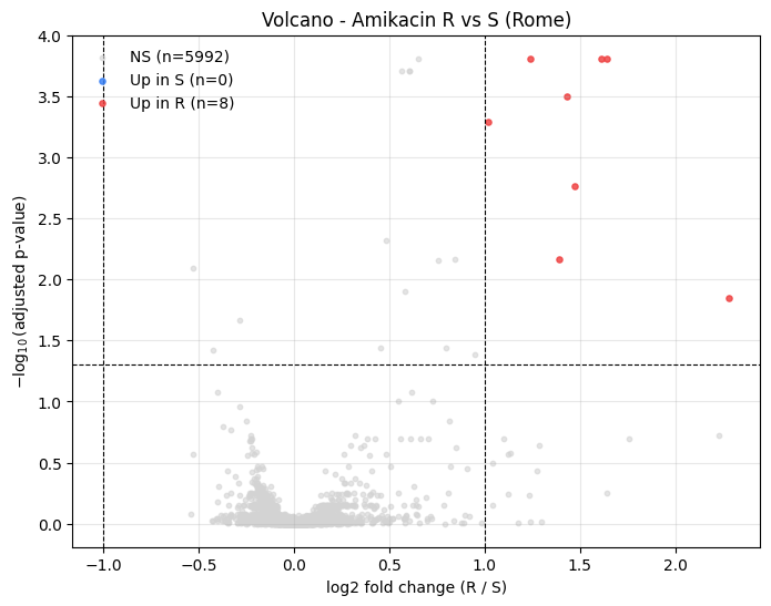
Volcano Plot

plot_volcano shows log2 fold change on the x axis and -log10(adjusted p-value) on the y axis. Points are coloured by direction:

• red: up in resistant (fold_change > fc_threshold and adj.p <= p_threshold)

• blue: up in susceptible (fold_change < -fc_threshold and adj.p <= p_threshold)

• grey: non-significant

from maldiamrkit.differential import plot_volcano

_ = plot_volcano(
    analysis.results,
    fc_threshold=1.0,
    p_threshold=0.05,
    title="Volcano - Amikacin R vs S (Rome)",
)

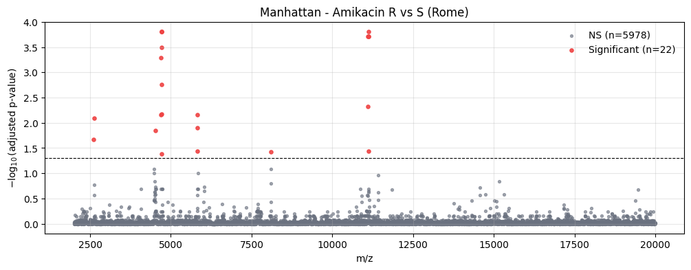
Manhattan Plot along the m/z Axis

plot_manhattan places each bin at its m/z position and plots -log10(adjusted p-value). Points above the dashed line pass the significance threshold.

from maldiamrkit.differential import plot_manhattan

_ = plot_manhattan(
    analysis.results,
    p_threshold=0.05,
    title="Manhattan - Amikacin R vs S (Rome)",
)

Compare across Multiple Drugs

DifferentialAnalysis.compare_drugs returns a boolean matrix whose rows are the union of significant m/z bins across all drugs and whose columns are drug names. True means the peak is significant for that drug.

We use the two antimicrobials annotated in MALDI-Kleb-AI - Amikacin and Meropenem - which share isolates but have different resistance mechanisms, so the overlap between their significant-peak sets is interesting on its own merits.

ds_mero = load_maldi_kleb_ai(antibiotic="Meropenem", verbose=False)
encoder_nan = LabelEncoder(intermediate="nan")
y_mero = (
    pd.Series(
        encoder_nan.fit_transform(ds_mero.meta["Meropenem"]),
        index=ds_mero.meta.index,
        name="Meropenem",
    )
    .dropna()
    .astype(int)
)
X_mero = ds_mero.X.loc[y_mero.index]

analysis_amk = DifferentialAnalysis(X, y).run()
analysis_mer = DifferentialAnalysis(X_mero, y_mero).run()

comparison = DifferentialAnalysis.compare_drugs(
    {"Amikacin": analysis_amk, "Meropenem": analysis_mer},
    fc_threshold=1.0,
    p_threshold=0.05,
)
print(f"Union of significant bins: {len(comparison)}")
print("Per-drug counts:")
print(comparison.sum())

Union of significant bins: 14
Per-drug counts:
Amikacin      8
Meropenem    13
dtype: int64

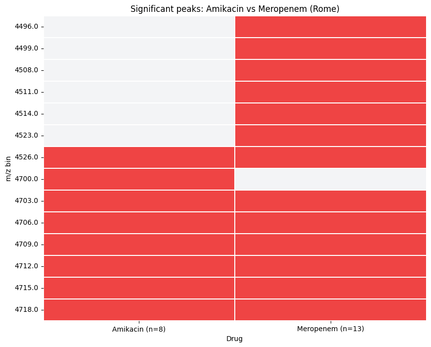
Boolean Heatmap

plot_drug_comparison(..., kind='heatmap') renders a compact peaks x drugs matrix - useful for spotting drug-specific peaks at a glance.

from maldiamrkit.differential import plot_drug_comparison

_ = plot_drug_comparison(
    comparison,
    kind="heatmap",
    title="Significant peaks: Amikacin vs Meropenem (Rome)",
)

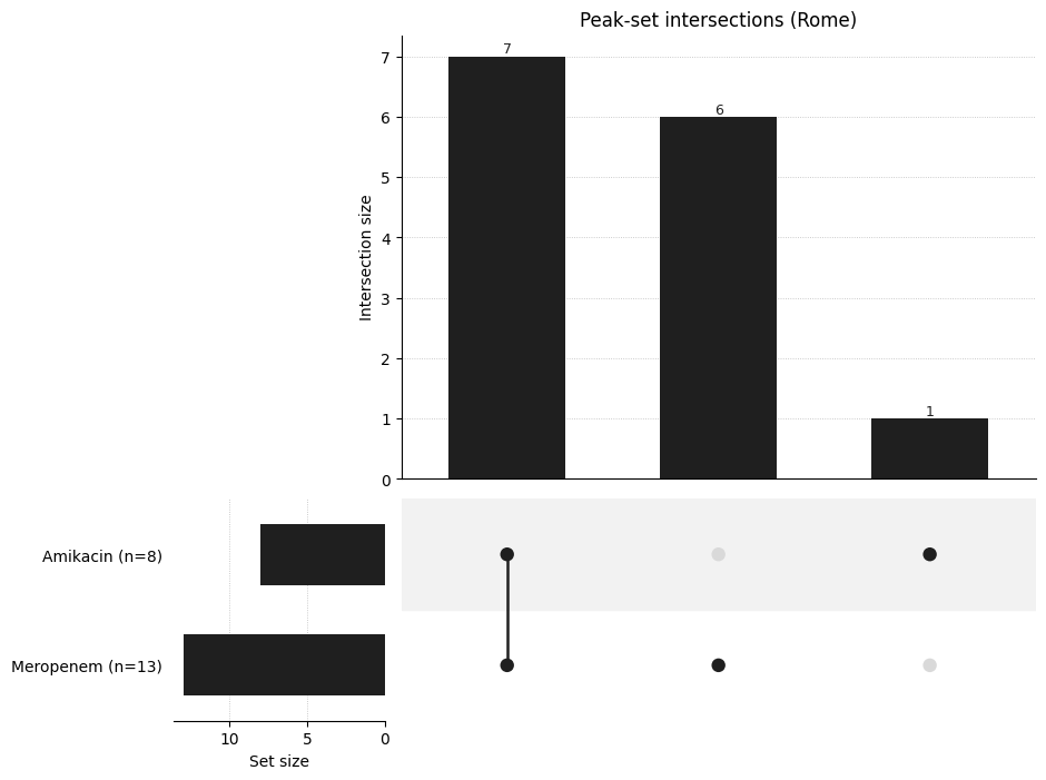
UpSet-style Intersection Plot

With more drugs, a Venn diagram stops scaling - an UpSet plot shows the size of every intersection of significant-peak sets.

_ = plot_drug_comparison(
    comparison,
    kind="upset",
    title="Peak-set intersections (Rome)",
)

Choosing a Test and Correction

DifferentialAnalysis.run() accepts both plain strings and the StatisticalTest / CorrectionMethod.

StatisticalTest enums:

test	When to use
mann_whitney	Default. Non-parametric, robust to MALDI intensity distributions.
t_test	Welch’s t-test (unequal variances). Use for approximately-Gaussian data.

CorrectionMethod enums:

correction	Meaning
fdr_bh	Benjamini-Hochberg FDR. Good default.
fdr_by	Benjamini-Yekutieli FDR. More conservative under dependence.
bonferroni	Family-wise error control. Most conservative.

Example of a conservative configuration:

analysis_strict = DifferentialAnalysis(X, y).run(
    test="t_test",
    correction="bonferroni",
)
analysis_strict.top_peaks(n=5)

	mz_bin	mean_r	mean_s	fold_change	p_value	adjusted_p_value	effect_size
3038	11114.0	0.000125	0.000080	0.652812	2.290201e-11	1.374120e-07	0.589519
905	4715.0	0.000506	0.000162	1.642962	9.656653e-11	5.793992e-07	0.546662
3039	11117.0	0.000127	0.000083	0.604224	2.661767e-10	1.597060e-06	0.558619
901	4703.0	0.000284	0.000120	1.241332	4.082946e-10	2.449768e-06	0.522023
3037	11111.0	0.000102	0.000067	0.604420	4.436762e-10	2.662057e-06	0.545698

Optional: Scoping Filters

When you already know which m/z regions matter, or you want to limit the hypothesis burden, pass mz_ranges and/or peak_detector to run():

from maldiamrkit.detection import MaldiPeakDetector

scoped = DifferentialAnalysis(X, y).run(
    mz_ranges=[(3000, 6000), (9000, 12000)],
    peak_detector=MaldiPeakDetector(method="local", binary=True, prominence=1e-4),
)
print(f"Bins tested (scoped):   {len(scoped.results)}")
print(f"Bins tested (full run): {len(analysis.results)}")
print(f"#adj <= 0.05 (scoped):  {(scoped.results['adjusted_p_value'] <= 0.05).sum()}")

Bins tested (scoped):   1994
Bins tested (full run): 6000
#adj <= 0.05 (scoped):  23

See Also

• API Reference - Differential

• Exploration notebook for PCA, t-SNE, UMAP, and spectral similarity